Protecting Cells

Sometimes there are sheets that you want to share, but maybe some of the data needs to be fixed.  This is when protecting cells can help. 

To protect a cell or a range of cells:

1. Highlight the cell or cells and select the DATA menu.

2. In the DATA menu, select, Protect sheets and ranges

3. In the menu that appears on the right, enter a description. In my example, I wrote a message for whom to contact for editing rights.

4. You can also change permissions and add a warning when clicking the cell. You can also add collaborators who are able to edit the data without a warning. To do this click the Change permissions  button below the range.

After clicking Change permissions, this pop-up appears.

5. To delete a protected range, open the right-side menu again by clicking on DATA and Change permissions. 

Click on the trash can.

Working on Putting Together Email Addresses

My coding club has a spreadsheet of student accounts. Each account needs me to make an individual email address. Fortunately, they all follow the same pattern

firstname.lastname@ymca.ca

The first formula I tried was TEXTJOIN. 

This formula =TEXTJOIN(".",TRUE,A141,B141,"@ymca.ca"), gave me the following.

Firstname.Lastname.@ymca.ca

Then I needed to change the capital letters to lowercase, so I used the LOWER function, =LOWER(I139), which gave me

firstname.lastname.@ymca.ca

Looking for a way to remove the period after "lastname", I tried the SUBSTITUTE function, =SUBSTITUTE(I140," ","."), which gave me the following result.

firstname lastname @ymca.ca

Frustrated, I Googled the answer.

SOLUTION

The CONCAT function.

Solution Page

Add Cells From a Different Sheet

I teach a coding course where some of my lessons have combined classes come to me. We recently had some new students and I wanted to see what the updated number of students in the class would be. 

I started by simply adding the numbers. I found that you can hold CMD and click on all the cells and Google Sheets will automatically give you the sum of the numbers.

But what happens when students enter or leave the school? I have to manually update my sheets. 

Fortunately, I have access to the main spreadsheet with the class numbers. 

Since I want an up-to-date sheet, I knew I could use the IMPORTRANGE function to get the information. Then I needed to add them together using the SUM function. 

The final formula looked like this below.

=SUM(IMPORTRANGE("sheetURL", "Sheet!C28:C29")+IMPORTRANGE("sheetURL", "Sheet!C30:C31"))

RANDBETWEEN Function

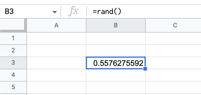
The RAND function in Google Sheets will give you a random number. 

=RAND()

As you can see in the above screenshot, the RAND function will probably not give you a usable number right away. That is where the RANDBETWEEN function comes in. With RANDBETWEEN, you can set the parameters of the integers (whole number)  you are interested in seeing. In the example below, RANDBETWEEN will choose between 1 and 10.

The RANDBETWEEN function can be used with text as well. Below is an example of using the RANDBETWEEN function with a list of names. 

By combining the INDEX function with RANDBETWEEN, it is possible to find a random name in a list. 

STEPS

1. Paste or type your list of names or words.

2. Type INDEX and choose the range of the list. In my example, the range is A29:A33.

3. After the range, type a comma.

4. Type RANDBETWEEN with the lower limit of the list (1) and the upper limit. Since I have 5 names, my upper limit is 5.

Instead of having a list as in the above example, the list of names can be added directly into the formula by putting them in curly braces {}.

If the data will change often, it might be better to simply use the cell names to use RANDBETWEEN. 

Interactive Chart Data with Checkboxes

Data is most useful when it can be manipulated easily, by anyone. 

To help our admissions officer, I made a checklist of countries where our current students have come from. I made this last school year, so I am trying to reconstruct this.

I must have started by taking the student data and putting it on the first sheet. Again, I am just guessing, but that seems like a reasonable place to start.

Then, I am pretty sure I followed that by starting building the formulas on the second sheet. I made three columns, a country name, number of students for that country, and then the checkbox. 

The formula I used was a SUMIFS formula 

=IF(C2,SUMIFS(Sheet1!$B27:$B51,Sheet1!$C27:$C51,A2),0)

This formula made it so that the student population would show up only when the box was checked. I then made a chart from the column with the number of students. That way when the numbers changed, the chart also changed in real time.

I would like to make it so that when you are looking at the chart of all the students, you could check a box and that would pull out the piece of the chart you were looking at.

Display a Value From Another Sheet

If you have ever wanted to display a value from another sheet, IMPORTRANGE is the formula for you.

Translate in Sheets

Last week I watched my coworker cut and paste responses from a spreadsheet to Google Translate and back again. It seemed like a tedious process that I knew had to have an easier solution. And if there wasn't, I thought that could be a solution an extension or addon could solve.

A Google Search away, I found that Google Sheets has a TRANSLATE forula built in. I remember hearing about it a few years ago, but I forgot about it until now.

The Documentation from Google is here.

The basic idea is this:

GOOGLETRANSLATE(text, [source_language, target_language])