RANDBETWEEN Function

The RAND function in Google Sheets will give you a random number. 

=RAND()

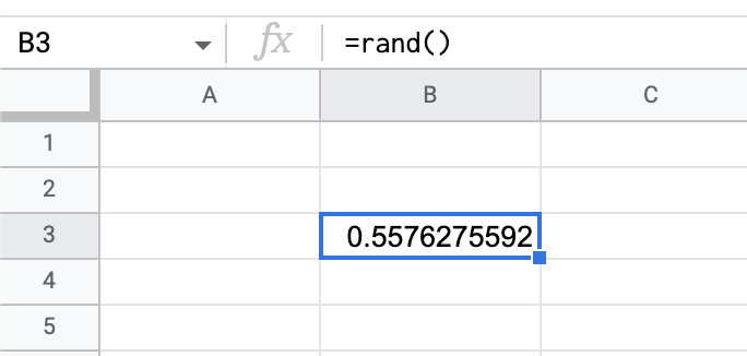
As you can see in the above screenshot, the RAND function will probably not give you a usable number right away. That is where the RANDBETWEEN function comes in. With RANDBETWEEN, you can set the parameters of the integers (whole number)  you are interested in seeing. In the example below, RANDBETWEEN will choose between 1 and 10.

The RANDBETWEEN function can be used with text as well. Below is an example of using the RANDBETWEEN function with a list of names. 

By combining the INDEX function with RANDBETWEEN, it is possible to find a random name in a list. 

STEPS

1. Paste or type your list of names or words.

2. Type INDEX and choose the range of the list. In my example, the range is A29:A33.

3. After the range, type a comma.

4. Type RANDBETWEEN with the lower limit of the list (1) and the upper limit. Since I have 5 names, my upper limit is 5.

Instead of having a list as in the above example, the list of names can be added directly into the formula by putting them in curly braces {}.

If the data will change often, it might be better to simply use the cell names to use RANDBETWEEN.