RANDBETWEEN Function

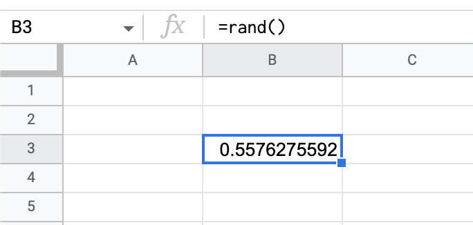
The RAND function in Google Sheets will give you a random number. 

=RAND()

As you can see in the above screenshot, the RAND function will probably not give you a usable number right away. That is where the RANDBETWEEN function comes in. With RANDBETWEEN, you can set the parameters of the integers (whole number)  you are interested in seeing. In the example below, RANDBETWEEN will choose between 1 and 10.

The RANDBETWEEN function can be used with text as well. Below is an example of using the RANDBETWEEN function with a list of names. 

By combining the INDEX function with RANDBETWEEN, it is possible to find a random name in a list. 

STEPS

1. Paste or type your list of names or words.

2. Type INDEX and choose the range of the list. In my example, the range is A29:A33.

3. After the range, type a comma.

4. Type RANDBETWEEN with the lower limit of the list (1) and the upper limit. Since I have 5 names, my upper limit is 5.

Instead of having a list as in the above example, the list of names can be added directly into the formula by putting them in curly braces {}.

If the data will change often, it might be better to simply use the cell names to use RANDBETWEEN. 

Interactive Chart Data with Checkboxes

Data is most useful when it can be manipulated easily, by anyone. 

To help our admissions officer, I made a checklist of countries where our current students have come from. I made this last school year, so I am trying to reconstruct this.

I must have started by taking the student data and putting it on the first sheet. Again, I am just guessing, but that seems like a reasonable place to start.

Then, I am pretty sure I followed that by starting building the formulas on the second sheet. I made three columns, a country name, number of students for that country, and then the checkbox. 

The formula I used was a SUMIFS formula 

=IF(C2,SUMIFS(Sheet1!$B27:$B51,Sheet1!$C27:$C51,A2),0)

This formula made it so that the student population would show up only when the box was checked. I then made a chart from the column with the number of students. That way when the numbers changed, the chart also changed in real time.

I would like to make it so that when you are looking at the chart of all the students, you could check a box and that would pull out the piece of the chart you were looking at.

Display a Value From Another Sheet

If you have ever wanted to display a value from another sheet, IMPORTRANGE is the formula for you.

Translate in Sheets

Last week I watched my coworker cut and paste responses from a spreadsheet to Google Translate and back again. It seemed like a tedious process that I knew had to have an easier solution. And if there wasn't, I thought that could be a solution an extension or addon could solve.

A Google Search away, I found that Google Sheets has a TRANSLATE forula built in. I remember hearing about it a few years ago, but I forgot about it until now.

The Documentation from Google is here.

The basic idea is this:

GOOGLETRANSLATE(text, [source_language, target_language])

Formatting Numbers

A while back I was asked how to make all phone numbers in a list the same format. I don't have a very good solution, but I have something.

The first idea I had was to do data validation in the Google Form where you collect the data. Getting data as pure as you can when you collect it is always the best.

But the information had already been collected.

Step 1

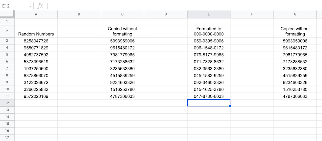
The first thing I wanted to do was to see if I could get a list of random numbers. Fortunately, Google Sheets has a RAND function that will do just that.

Step 2

Step 2 was to copy the numbers without formatting. When you paste into Google Sheets, there is a little clipboard icon that shows up. Clicking that will give you the option for a menu where you can choose to paste the values or the formatting. I chose the values because I didn't want the function anymore. Besides being good practice, the RAND function would have kept changing the data.

Step 3

The next thing I did was to reformat the numbers. I went to format > number > custom number format. Then I put in the formatting for a Japanese cell phone. (In my example another recommendation was to make a separate field in the form for a home telephone number that has a different formatting.)

Make an Escape Room Activity with Google Sheets

 

Click to make a copy

I saw a Google sheet that had math problems and if you got the problems right it revealed the image. I was tempted to buy the sheet on TPT, but I thought I could do it myself.

In my first attempt a few weeks ago, I didn't get anything to work. 

But after a few hours this morning, I got it. Here is my flow.

Steps to make it
1. First I searched for [google sheets reveal image]. 

2. I found this site https://sheetshelp.com/image/

3. I scanned the article and went to the comments. 

4. The first comment talks about basing an image on another cell and the author's reply gave a link to a support document.

5. The support document was for the function IFS (which means two IF statements) but I wanted one. So I went to the support page for the IF function.

6. I got the syntax for the IF function.

7. I found an image I could use. I wasn't picky so I went to Pixabay and looked for an open picture of a robot. 

8. I thought I could cut it into 9 pieces using GIMP (open source Photoshop), so I searched for something like [cut image into equal parts GIMP].

9. Then I looked for an online editing site that could do it for me.

10. I found one and cut my image into 9 parts.

11. Then I uploaded my 9 images to Google Drive.

12. I put the images in a folder on Google Drive and tried to link to them.

13. Despite changing the link settings, it didn't work. It also didn't work on Dropbox and Box. None of the three give a URL with the ending being .png or .jpg.

14. I published the images to a Blogger post and copied the image URL.

15. I did a test of the IF function.

16. I got it to work with both TRUE and FALSE values.

17. Then I tried it with an image. But it didn't work.

18. It didn't work because I had the equal sign in front of IMAGE. I fixed it and got: =IF(A3=1,IMAGE("https://i.creativecommons.org/l/by/4.0/88x31.png"),"green")

19. With the images working in the formula, I added my own images.

20. They were not cut right so I had to go back to the online image site and redo them.

21. The robot was not lining up so I had to make those three columns narrower.

22. The sheet was too busy so I made a new sheet and cleaned it up.

I can see using this as a digital breakout room and it can be used in any subject. I suggested to my wife that she use it in her Japanese class. She could start with just having the students complete the sheet, then each time you did it, show them how you made it little by little. She teaches HS, so they could totally make something like this.

Click the above image for a template of my work.