Creating Vertical Lists with Checkboxes

 =TEXTJOIN(CHAR(10), TRUE, FILTER(B4:B5, C4:C5=TRUE))

Today, I realized you can use a formula to make a list inside a cell in Google Sheets. 

Why would you want to do this?

In my case,  I am trying to make the IEP/ILP process smoother. It doesn't make sense to keep rewriting information each time you write a report about a student. I think using a Google Sheet to make a document will be easier. 

I was able to put text together using TEXTJOIN and separated by a space or by comma before, but ChatGPT showed me that I could add the CHAR(10) -- line break -- to a formula to make the list.

This formula puts checkmarks in a list, in order of day, combined with the labels from the matrix.

Save this formula for later. 

=TEXTJOIN(CHAR(10), TRUE, ARRAYFORMULA(IF(B81:F86, A81:A86 & " " & B80:F80,)))

I ended up separating them out into the columns to the right of the checkboxes.

Challenge Accepted

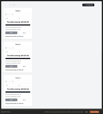
A few weeks ago, maybe a few months now, I created a schedule using ClaudeAI to make a testing clock. 

It's functional. It works. 

Today I noticed that my colleague, who also does testing accommodations, had a spreadsheet projected on the whiteboard with the times.

When he projects it on the whiteboard, it looks like this:

I asked about the formulas in it. At the time, he didn't have any. 

My mind immediately went to work about how to make it work in Google Sheets. 

I had the basic structure in my mind. During my break I went to work building it. 

When we give accommodations, we write the start time, 30 minutes remaining, 5 minutes remaining, and the end time. Calculating this is always a chore. 

To the spreadsheet! 

I knew I wanted a drop-down of student names. This would eventually be for all students in inclusion support, so it would be quick and easy to use.

I found online that I could use a formula called =TIME. Using ChatGPT, I was able to do a VLOOKUP with all the names that looks like this - =B4+TIME(0,B3,0)+TIME(0,B8,0)

Here are all my formulas for this one.

=B7-TIME(0,5,0)

=B7-TIME(0,30,0)

=B4+TIME(0,B3,0)+TIME(0,B8,0)

=B3 + (B3 * IFERROR(VLOOKUP(B1, E4:F7, 2, FALSE), 0))

My tool

Here's a link to the working example.

https://docs.google.com/spreadsheets/d/15FjeNAyHnTran4ejfxk4M477AJrGNJFjxo6P_m2VpZI/edit?gid=1058096702#gid=1058096702

I'll start making it look better tomorrow. I also have to check my formulas.